Table of Contents

Previous: 4. Logic Operations

Next: 6. Data Structures

5  Problem Solving with Computers

A high-level programming language usually supports data abstraction and control abstraction. In Chapter 2, we discuss representation and implementation of primitive data types. This Chapter and Chapter 6 will cover data abstraction of other complex data structures and other control abstraction such as for-loop, while-loop, and do-while-loop of C programming language. We begin with how to describe computational solutions using flowcharts and pseudo codes.

5.1  Flowchart and Pseudo Code

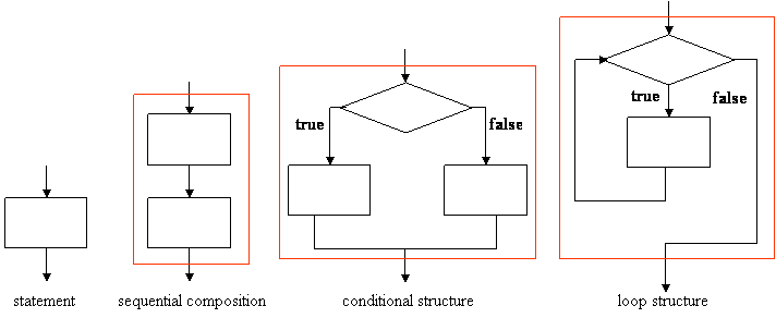
The control structures of a high-level programming language include four types: basic statement, sequential composition, conditional structure, and loop structure. These control structures are expressed using the following diagrams:

The rectangular box denotes a statement and the diamond box denotes a condition. These control structures have a common property, i.e., each of them has one entry point and one exit point. A basic statement is either an simple assignment or a composed statement in C programming language. A sequential composition is two statements connected by a semicolon (;) in C. A conditional structure is implemented as a if-then-else statement in C. A loop structure is implemented as a while-loop statement in C (in Section 5.5). The incoming arrow and outgoing arrow of the red box in the last three composed structures are the one entry point and the one exit point, respectively. The four basic control structures are called D-structure following from the originator Edsger W. Dijkstra (1930-2002).

The basic control  structure may be a single assignment statement or a function call such as x=y+z or printf("abc") as the two boxes below:

A sequence of statements connected by semicolons is using sequential composition. For example, x=y+z; y=z*100 can be expressed using the following flowchart. The two boxes are grouped together to become a large one-entry-one-exit control structure.

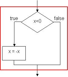
For conditional structure, we revisit the if-then statement of the absolute value:

The flowchart is depicted as the below that the statement in the false branch is absent.

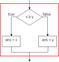
The if-then-else of the maximum function is:

which is described as the following flow chart:

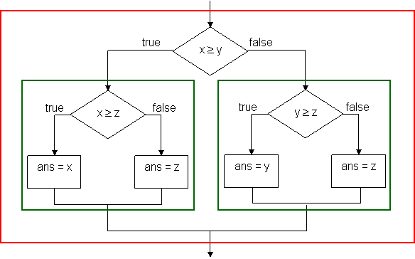
Nested conditional statements are drawn as multiple conditional structures. Recall the following program of computing the maximum of three variables using nested conditional statements.

The flowchart contains three conditional structures. Each of the two inner conditional structures are grouped together in the green boxes as two one-entry-one-exit statement and become the statement of the then branch and the else branch, respectively. The outer conditional structure is constructed as another one-entry-one-exit statement.

Next, let us consider the following program segment of switch-case statement with break statement in each case. The value of variable shape is  one of 'S', 'C', and 'T', denoting square, circle, and equilateral triangle, respectively, of a geometrical object. Variable d is either a side or a radius of the object according to the value of shape. The case clause assigns the perimeter or circumference of the object to m; for the other shapes, the program simply sets m to -1.

The program segment is usually described as the following flowchart:

This flowchart is not constructed by the four one-entry-one-exit basic control structures. As mentioned before that a switch-case statement is equivalent to else-if construct. The program segment is rewritten as below:

The corresponding flowchart below is constructed by the four one-entry-one-exit basic control structures as below:

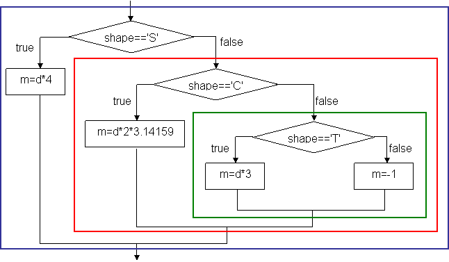
To solve a problem in computer, we must express the solution in a method that is suitable of implementation using the above control structures. First, a solution is written as a pseudo code. Let us recall the stepwise conversion of a decimal integer to a binary numeral in Section 2.2:

We can draw the following flowchart for the above pseudo code:

Function concat(b,d) is to append d at the left-hand-side of b. The above flowchart is, in fact, equivalent to the following flowchart which is constructed by the four types of one-entry-one-exit control structure:

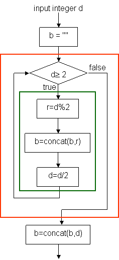
The statements in the green box are sequentially composed as a block statement. The while-loop in the red box is composed to form a one-entry-one-exit statement. According to the modified flowchart, the pseudo code is rewritten to:

The flowchart and pseudo code can be easily implemented as a C program. We show the implementation of converting a decimal integer to a binary numeral in next section. Flowcharts and pseudo codes are used to design solution of computing problems. We will continue to explain algorithms of searching and sorting problem in the following sections.

5.2  Arrays and Iterations in C

One-Dimensional Arrays

An array is a data structure of C programming language that is used to specify an aggregation of homogenous data elements. The syntax of an one-dimensional array declaration is:

where the value integer must be a positive number or a variable with positive value. For example, the examination scores of a class of ten students is declared as:

n array can be declared with initial values.

Array score contains ten cells that each holds an integer element with the following initial values:

An array can also be partially initialized. For example, the following array declaration assigns initial values to score[0], score[1], score[2], score[3], score[4], score[5], and score[6]. Also, data elements score[7], score[8], and score[9] are set to zero's.

In C programming language, access of array elements are through the identifier of an array and an index. For an array of n elements, the indices of its elements range from 0 to n-1. Therefore, array score has ten elements and the indices range from 0 to 9. The first element of array score is score[0], the second element score[1], etc. An array element can be modified with an assignment statement:

With the above two assignments, array score is changed to:

Array elements can be used in arithmetic expressions. The following statement assigns the average score to variable average:

 Suppose the address register of a CPU is 32-bit long and the the size of an integer is four bytes. If the starting address of score[0] is 0x22FF50, the array elements socre[1], score[2], ¼, and score[9] are stored in the succeeding memory locations, i.e., the starting address of score[1] is 0x22FF54, the starting address of score[2] is 0x22FF58, ¼, and the starting address of score[9] is 0x22FF74. The addresses (in hexadecimal) of array elements score[i] are shown as the figure below:

In C programming language, the identifier of a one-dimensional array represents the address of the first array element. For example, in program array_value_address_1D.c, Lines 6 and 7 output the content of array score and address of score[0], i.e., 0x22FF50. Lines 9 and 10 prints the values of *score and score[0], where both values are 78. The notation *score is dereferencing of score once. C programming language also allows arithmetic operation of address. In Line 12, score+2 is an arithmetic operation of address which means the address of score adds two times of the size of a given data type, that is 4 for the integer type. Hence, score+2 is equivalent 0X22FF50+4*2 which is exactly the address of score[2], 0X22FF58, as the output of Line 13. Lines 15 and 16 prints the values of *(score+2) and score[2], where both results are 90.

The output of program array_value_address_1D.c is as below:

In general, let the starting address of array a[n] be loc and the type of the elements of a[n] be T. We have the address of &a[0]==loc and the starting address of array element a[i] is given as, since there are i elements before a[i] and each element occupying sizeof(T) bytes:

a+i = &a[i] = loc + sizeof(T) ´ i.

Multi-Dimensional Arrays

Arrays in C programming language can be declared with multiple dimensions. The syntax of two-dimensional array is:

where integer1 and integer2 must be positive numbers or variables with positive values. A two dimensional array is actually a one-dimensional array of integer1 elements such that each element is a one-dimensional arrays of size integer2 of the specified type type. Consider the following two-dimensional array declaration:

Array data is a one-dimensional array of three elements data[0], data[1], and data[2] such that each element is a one-dimensional array of four elements. There are two ways to initialize a two-dimensional array in array declaration: (1) with a one-level list of numbers enclosed by curly brackets and (2) with a two-level list enclosed by curly brackets such that the first level elements are lists of numbers enclosed by curly brackets. Examples of array initialization are:

The diagram of array data[3][4] is depicted in the following figure:

Program array_value_address_2D.c is an example to explain the expressions of value and address of multi-dimensional array. There are six cases of value and address expressions. We will explain each case separately.

Lines 9 to 14 of Case 1 print the location of six expressions. Expression &data (Line 9) is the address of array data. Expression data (Line 10) is the contents of array variable data, which is a pointer to the address of one-dimensional array data[0]. This address is expressed as &data[0] (Line 11). Expressions *data and data[0] (Lines 12 and 13) are the content of data[0], which is a pointer to the address of one-dimensional array data[0][0], i.e., &data[0][0] (Line 14). In C programming language, these expressions point to the same location, e.g., 0X22FF50, the starting address of the array elements.

Lines 17 to 19 of Case 2 print values of three expressions, **data, *data[0], and data[0][0] all yield the value of array element data[0][0] which is 12.

Lines 22 to 26 of Case 3 print location of five expressions. Expression data+1 (Line 22) is calculated using pointer arithmetic. Expression data is a pointer to the address of one-dimensional array data[0]. Since an element of data[0] is a one-dimensional array of four elements, it is of size 16 bytes. Therefore, data+1 the location of data[0] adding the size of its element, i.e., 0X22FF50+0X10=0X22FF60. The location is exactly the  address of expression &data[1] (Line 23). Lines 24 and 25, *(data+1) and data[1] are the content of data[1] which is the address of array element data[1][0] (Line 26).

In Lines 29 to 31 of Case 4, the three expressions **(data+1), *data[1], and data[1][0] all refer to the value data[1][0] which is 31.

Lines 34 to 36 of Case 5 all print the address of data[1][2]. Since expressions *(data+1) and data[1] are the address of data[1][0], expression *(data+1)+2 and data[1]+2 are the address of data[1][0] adding the size of two integer elements, i.e., data[1][0]+4*2=0X22FF68, that is the address of data[1][2].

Finally, Lines 40 to 42 of Case 6 print the value of data[1][2] which is 30.

In general, let the starting address of two-dimensional array a[m][n] be loc and the type of the elements of a[m][n] be T. Let us view array a[m][n] as the following m´n matrix:

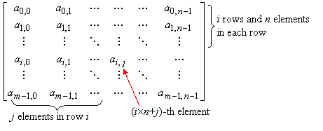
Suppose the matrix elements are stored in memory in the row-major order. Recall that the matrix indices starts from (0,0), There are i rows before element a_i,j such that each row has n elements, and there are j elements in row i before element a_i,j. Totally, there are i´n+j elements, that each element is of sizeof(T) bytes, in front of a_i,j. We have the address of &a[0][0]=loc and the starting address of array element a[i][j] is given as:

*(a+i)+j = a[i]+j = &a[i][j] = loc + sizeof(T) ´ (i ´ n + j).

Let the starting address of three-dimensional array a[m][n][p] be loc and the type of the elements of a[m][n][p] be T. Let us view array a[m][n][p] as the following m matrices of size n´p:

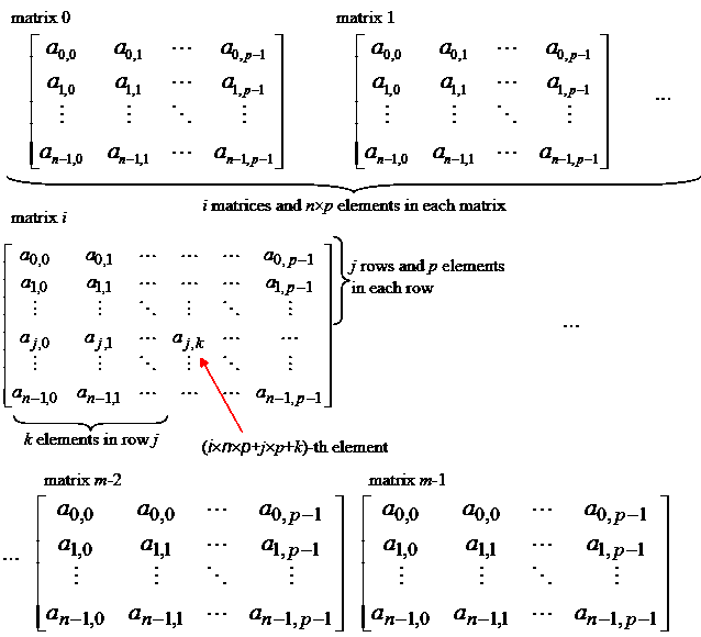
Suppose the matrix elements are stored in memory in the row-major order. Recall that the matrix indices starts from (0,0,0), There are i matrices, of size n´p, before the one containing matrix i. In matrix i, there are j rows before element a_j,k such that each row has p elements, and there are k elements in row j before element a_i,j. Totally, there are i´n´p+j´p+k elements, that each element is of sizeof(T) bytes, in front of a_j,k of matrix i. We have the address of array a is &a[0][0][0]=loc and the starting address of array element a[i][j][k] is given as:

&a[i][j][k] = loc + sizeof(T) ´ (i ´ n ´ p + j ´ p + k).

In C programming language, an array can be declared with reserved word static as well. If an array is declared with static, the memory space of the array will be allocated statically and it is called a static array; if an array is declared without static, the memory space of the array is allocated in a data structure called runtime stack and it is called a stack-dynamic array. Also, an array can be declared without specific array size, e.g., int a[ ][ ]. The size of array a is determined during program execution and its memory space will be allocated dynamically during program execution, too. We will discuss details of dynamic arrays in Section 8.3.

Definite Loops

However, it would be tedious and difficult to write such an assignment, if there are a great number of students, say, 100. Most high-level programming language, including C, provides loop constructs to accomplish such a computation. The first loop construct is for-loop with the following syntax:

The first part initiator is an assignment or a sequence of assignments that initialize some variables called loop variables. The second part condition is a loop condition which is evaluated at the beginning of every iteration. If the loop condition is true than the body statement will be executed; otherwise execution of the loop terminates. The third expression modifier is an assignment or sequence of assignments that modify the values of loop variables at the end of every iteration. Note that initiator, condition, and modifier are separated by semicolons (;). If initiator, condition, or modifier has more than one statements or expressions, the statements and expressions are separated by commons (,). A for-loop can be drawn as the following one-entry-one-exit control structure:

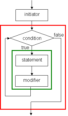
In the above flowchart, initiator is evaluated before the loop and condition becomes the loop condition, and statement and modifier make up the loop body.

For example, program average_score.c uses a for-loop to accumulate the total score of ten students. In Line 8, variable i is used as the loop variable which is initialized to zero in the first expression i=0. The loop condition in the second expression is i<10 that is the range of array index 0 to 9. The third expression is the modifier which increments the loop variable by 1. Line 9 is the loop body. Since the loop body contains a single statement, it is not enclosed by a pair of curly brackets. Using loop construct, it is easy to write a program to compute the average score of  100 students or larger. We simply change the loop condition according to the number of students.

The output of the average score is:

We show another program highest_score.c that reads the scores of ten students and set the highest score to variable max. The first for-loop reads the scores and the second for-loop set the highest score.

The input of scores and the output of the highest score is:

Indefinite Loops

An indefinite loop is a loop whose loop body will be executed as long as its loop condition holds. Hence, it is difficulty to tell exactly how many iterations will be executed for an indefinite loop. C programming language supports two kinds of indefinite loops: while-loop and do-while-loop. The syntax of while-loop is:

The semantics of while-loop is to evaluate condition first. If condition is evaluated to true (a value other than zero), statement will be executed. When execution of statement completes, repeat the while-loop. Once condition is evaluated to false (zero), the while-loop terminates. Hence, while-loop is exactly the one-entry-one-exit control structure.

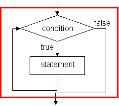
If condition of a while-loop is equivalent to true, the loop is a non-terminating loop or an infinite loop. For example, the following loop is an infinite loop because x+1>x is always true.

If condition of a while-loop is equivalent to false, the loop does not have any computational effect. For example, the following loop is equivalent to no operation because the x+1==x is always false.

Program character_scan_while.c reads one character a time up to 30 characters or encountering a terminating character '|'. Then the character string is printed. Note that function call scanf("%c", &c[i]) in this program reads a single character including space, tab, line feed, carriage return control characters, and non-printable characters. Since it is not known how many characters will be scanned, an indefinite while-loop is used. The loop will terminate when 30 characters are scanned or the vertical bar '|' is scanned.

The syntax of do-while-loop is:

The semantics of do-while-loop is to execute statement and then to evaluate condition. If condition is evaluated to true, repeat the do-while-loop; otherwise the loop terminates. Unlike while-loop, the loop body statement of do-while-loop is executed at least once. In fact, do-while-loop is equivalent to the following program construct:

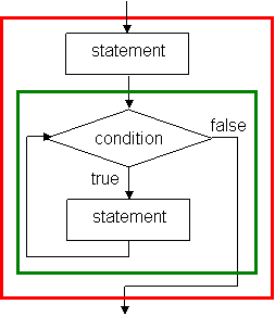
Program character_scan_while.c reads at least one character. It is easier to rewrite this program using do-while-loop. Note that there is a minor difference that the program below, character_scan_do_while.c, will output the terminating character '|', if the number characters is less than 30.

In the rest of this chapter, we will explain problem solving and programming design with computers using searching and sorting as examples.

5.3  Sequential Search

Suppose a sequence of data are stored in a one-dimensional array, say, a[n]. The search problem is to find whether a specific data value, say, key, is an element of the data sequence and to determine which element is the specific data value if it exists. Let us assumed the sequence is stored in the arbitrary order. When we solve a problem, it is important to figure out a way, or called an procedure, that will achieve the goal of the problem effectively. For example, an easy way to carry out the search is to pick up a data element in a[i], where 0£i<n, randomly and check if a[i] is of value key. Repeat this process until an element with value key is found or all the elements are checked.

Since we are going to solve a problem with a computer, it is also important that the solution must be a stepwise procedure that can be understood or be performed on a computer. A stepwise procedure that can be performed on a computer is called an algorithm. For example, the above searching procedure needs to be refined further to become a searching algorithm: (1) how to pick up an element a[i] randomly, and (2) how to make sure all elements have been checked, if key is not an element of a[n]. To refine the procedure, we can do the following steps:

1. Use a random number generator, which is supported by most programming language such as C,  to decide which element to check.

2. Mark the elements that have been checked. This can be done by using another array, say, checked[n], to store the marker.

However, the computation of random number generation is costly and the use of an additional array also consumes memory space. We may modify the procedure in a much easier way: check the elements starting from a[0], then a[1], a[2], and so on, until key is found or a[n] is reached. The modified steps can be written as the following pseudo code:

This search algorithm is known as sequential search algorithm. We draw the flowchart of sequential search algorithm as the following:

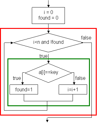
At the end of this flowchart, if found==1 then the search succeeds and a[i] is element being found; otherwise, the search fails. Program sequential_search.c is a program implementing the sequential search algorithm. An integer array of eight elements is used to illustrate the sequential search algorithm. Lines 10 to 16 are the statements corresponding to the implementation of the flowchart. Lines 18 and 19 reports the searching result according to the value of found.

Two runs of the program are shown below, one for successful search and another one for failed search:

Observing that if the value of a[0] equals to key, only iteration of the while-loop is executed; if all values from a[0] to a[n-2] do not equal to key, either a[n-1] equals to key or the search fails and n iterations of the while-loop are executed. In average, n/2 iterations are executed and we say the time complexity of the sequential search algorithm is n/2.

Program sequential_search_short_circuit.c is an alternative way to implement the sequential search algorithm. In the while-loop (Line 12), the loop terminates when i³8, search fails, or, a[i]==key, search succeeds. In the case of search failing, i is set to 8 and the second part of the loop condition will access a[8], which causes an error of segmentation fault, also known as array out of range. However, C programming language evaluates this condition using a technique called short-circuit evaluation to avoid the error.

Short-circuit evaluation is a technique that will return the result of an expression as soon as the result of the expression is determined by partial evaluation. For example, evaluation of condition pÙq will return false if p is evaluated to false and expression q is ignored; evaluation of condition pÚq will return true if p is evaluated to true and expression q is ignored. Hence, when i is 8, condition i<8 && a[i]!=key returns false without evaluating the second expression a[i]!=key.

5.4  Bubble Sort

Suppose a sequence of n elements are stored in a one-dimensional array, a[n]. The sorting problem is to rearrange the elements of a[n] so they are in ascending or descending order. We will present the pseudo code of bubble sort. The bubble sort algorithm has two nested loops. The outer loop deals partial sequences of a[n]. It starts from the entire sequence and, in each of the following iterations, the last element of the sequence is removed. The inner loop scans all elements of a given sub-sequence and selects the element with the maximum value. After the inner loop is completed, the selected element is swapped with the last element. Hence, at the end of the outer loop, the maximum value of the sequence is "bubbled" up to the right-most position of that sequence. We use variable max to record the current maximum value and inx to record the selected element.

The pseudo code is depicted as the following flowchart:

This flowchart is implemented as program bubble_sort.c as below:

The program sorts array data of ten elements. Lines 11 to 18 are the code for the bubble sort algorithm. The two loops are implemented as for-loops, instead of while-loops. Line 14 selects the maximum. Lines 15 to 17 swap data[inx] and data[i-1]. The output of the program is shown below:

The comparison operation of Line 15 is evaluated (n-1)+(n-2)+¼+1=n(n-1)/2 times. That is, the complexity of the bubble sort algorithm is n(n-1)/2.

5.5  Binary Search

The complexity of the sequential search algorithm is n/2. However, in many computer applications data are stored in sorted order. Searching in a sorted sequence can be accomplished in a much more efficient way using the binary search algorithm. The binary search algorithm tests the element in the middle. If it is the searched key, search is done successfully. If it is not the searched key and the middle element is greater than the searched key, then the left half of the sequence is searched; if the middle element is less than the searched key, the right half element of the sequence is searched. Each time an element is tested with unmatched result, half of the sequence is trimmed. Hence, it takes only log₂n comparisons to search a sequence of n elements. The pseudo code the binary search algorithm is given as below:

We leave the flowchart of the binary search algorithm as homework assignment and show the C program binary_search.c below:

Lines 10 to 15 are the program segment of the binary search algorithm. Two sample runs of the program are shown below:

Table of Contents

Previous: 4. Logic Operations

Next: 6. Data Structures